In this post I show how to conduct simple linear optimization in R. You can also find other posts written by me that look at other linear optimization tasks, suchs as the transportation problem (can be solved with lp.transport), the assignment problem (can be solved with lp.assign) and integer linear programming (also linear mixed integer problems can be solved in R).

Linear programming is widely applied for modelling facility location problems. lpSolve is an extension available in R providing access to an C-based interface for solving linear programming problems. Since the interface is developed in C it has maximum performance, minimizing the time required for solving linear programming problems without having to switch programming environment or programming language.

In this post I give an example of simple linear programming problem solved with lpSolve.

The objective function is to maximize revenue defined by the function f(x,y) = 2x + 3y, subject to the constraints that x, y are non-negative and x + y not greater than 3.

As the Internet will show you, this problem is easy to solve, i.e. by drawing a line plot or by applying the simplex algorithm. I will not explain the algorithms or methodology for solving linear problems in detail, but I will give a brief example of how this simple problem can be modelled and solved using lpSolve in R. Afterwards, I will show a graphical illustration which verifies the result.

I load the lpSolve package (having installed it already) and model the problem, using the lpSolve API:

library(lpSolve)
f.obj <- c(2,3)                           # coefficient vector of objective function
f.con <- matrix(c(1,1),nrow=1,byrow=TRUE) # coefficient matrix for constraint matrix
f.dir <- c("<=")                          # constraint direction vector
f.rhs <- c(3)                             # constraint values

Now let us solve the linear problem:

solution <- lp("max",f.obj,f.con,f.dir,f.rhs)
solution

## Success: the objective function is 9

The optimal solution is the following (optimal x and y value for problem at hand):

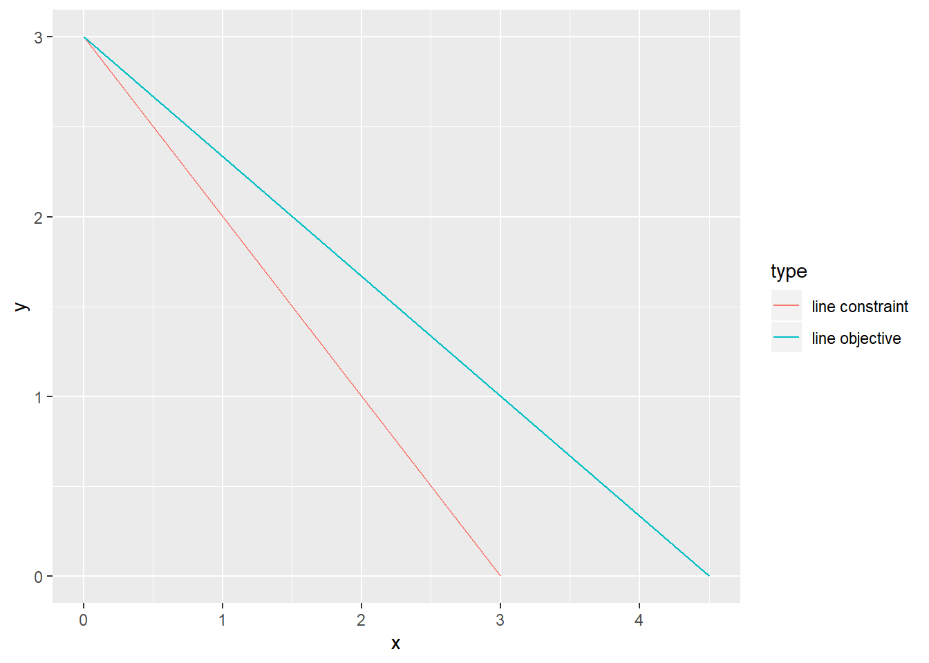
solution$solution

## [1] 0 3

Now let us graphically verify the result. I define two lines which I visualize using geom_line from the ggplot2 package. The first line represents the constraint that x + y must be no greater than 3, the second line represents the objective function. The line for the objective function represents it maximum achievable value, i.e. the optimal value. The line for the constraint represents its binding cases, i.e. when it equals exactly 3. In more simple terms: “line objective” : 2x + 3y = 9 “line constraint” : x + y = 3

library(ggplot2)
plot_df <- as.data.frame(matrix(nrow=4,ncol=3))
colnames(plot_df) <- c("x","y","type")
plot_df$x <- c(0,3,0,9/2)
plot_df$y <- c(3,0,9/3,0)
plot_df$type <- c("line constraint","line constraint", "line objective", "line objective")
ggplot(plot_df) + geom_path(mapping = aes(x=x,y=y,color=type))

Considering that x+y=3, can you see that the optimal solution to this problem must be x=0, y=3 – and that this maximizes the objective function?

If you are interested in non-linear programming (e.g. gradient descent with nloptr) or quadratic optimization (quadprog) in R, then please go ahead and check out my other posts on these types of optimization tasks too.