In a previous post I demonstrated how one can query automotive data via Quandl directly from within a Python script.

In this post I will document how to query platinum and palladium exchange prices from Quandl in Python. The data has been verified by London Palladium and Platinum market (http://www.lppm.com).

In the code below I retrieve a data set with platinum prices from Quandl

import quandl
# setting up API key
quandl.ApiConfig.api_key = "your key here"
import numpy
import pandas
# retrieving data from quandl in numpy format, then converting into pandas DataFrame
data = pandas.DataFrame(quandl.get('LPPM/PLAT', returns="numpy"))

The data set obtained includes daily opening and closing prices from metal exchange markets around the world. We can take a look at the header of the data frame obtained:

data.head()

	Date	USD AM	EUR AM	GBP AM	USD PM	EUR PM	GBP PM
0	1990-04-02	471.00	NaN	289.65	470.50	NaN	NaN
1	1990-04-03	475.80	NaN	291.35	477.25	NaN	NaN
2	1990-04-04	475.70	NaN	289.95	476.75	NaN	NaN
3	1990-04-05	481.75	NaN	292.60	481.85	NaN	NaN
4	1990-04-06	481.00	NaN	293.10	480.25	NaN	NaN

As can be seen the daily opening and closing prices are noted in USD, EUR, and GBP. Some of the columns are empty, however. Let us see if this is only the case for early entries by also checking the tail of the data frame retrieved:

data.tail()

	Date	USD AM	EUR AM	GBP AM	USD PM	EUR PM	GBP PM
7574	2020-03-30	721.0	650.43	581.45	726.0	658.80	585.25
7575	2020-03-31	723.0	657.87	586.61	727.0	662.72	586.53
7576	2020-04-01	723.0	660.27	585.19	714.0	653.25	576.04
7577	2020-04-02	727.0	665.75	585.35	727.0	668.20	585.82
7578	2020-04-03	719.0	666.05	584.55	714.0	662.34	582.62

For revent days prices were listed for all currencies. Since opening and closing prices were listed in USD both in 1990 and in 2020 I choose to focus on prices in USD only.

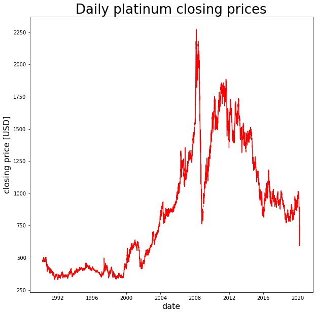
In the code below I plot platinum closing price history in USD, using matplotlib

import matplotlib.pyplot as plt
plt.figure(figsize = (10,10))
plt.plot(data["Date"], data["USD PM"],color = "red")
plt.title("Daily platinum closing prices",size=26)
plt.ylabel("closing price [USD]",size = 16)
plt.xlabel("date", size = 16)

Text(0.5, 0, 'date')

In the code below I repeat above workflow for palladium price history

First, I query the data from Quandl:

data = pandas.DataFrame(quandl.get('LPPM/PALL', returns="numpy"))

Next, I review the header of the data frame:

data.head()

	Date	USD AM	EUR AM	GBP AM	USD PM	EUR PM	GBP PM
0	1990-04-02	128.00	NaN	78.70	127.65	NaN	78.55
1	1990-04-03	128.35	NaN	78.60	128.50	NaN	78.75
2	1990-04-04	128.35	NaN	78.25	128.00	NaN	77.90
3	1990-04-05	128.40	NaN	78.00	127.75	NaN	77.65
4	1990-04-06	128.75	NaN	78.45	128.50	NaN	78.40

And I review the tail of the data frame too:

data.tail()

	Date	USD AM	EUR AM	GBP AM	USD PM	EUR PM	GBP PM
7574	2020-03-30	2236.0	2017.14	1803.23	2242.0	2034.48	1807.34
7575	2020-03-31	2317.0	2108.28	1879.92	2307.0	2103.01	1861.23
7576	2020-04-01	2314.0	2113.24	1872.93	2236.0	2045.75	1803.95
7577	2020-04-02	2288.0	2095.24	1842.19	2123.0	1951.29	1710.72
7578	2020-04-03	2234.0	2069.48	1816.26	2140.0	1985.16	1746.23

Again, I choose to focus on closing prices in USD. I plot the price history below, using matplotlib in Python:

plt.figure(figsize = (10,10))
plt.plot(data["Date"], data["USD PM"],color = "red")
plt.title("Daily palladium closing prices",size=26)
plt.ylabel("closing price [USD]",size = 16)
plt.xlabel("date", size = 16)

Text(0.5, 0, 'date')