이 글에서는 R의 회귀에 대한 다양한 예제를 제공한다. R을 이용한 다양한 회귀 방법을 비교한다. 소개할 방법은 단순 선형 회귀, 다중 선형 회귀, 다항식 회귀, 의사 결정 트리 회귀, 지원 벡터 머신 회귀이다.
R의 회귀에 필요한 패키지
필요한 패키지(R 기본 라이브러리에 추가)를 로드하여 시작합니다.
library(dplyr) # package for data wranglinglibrary(ggplot2) # package for data visualization
library(rpart) # package for decision tree regression analysis
library(randomForest) # package for random forest regression analysislibrary(e1071) # package for support vector regression analysis
library(caTools) # package for e.g. splitting into training and test setsR에서 회귀 전에 데이터 읽기
이제 R에서 회귀 예제를 구현하는 데 사용할 데이터를 읽었습니다. 데이터에는 국내 총생산, 총 민간 투자, 기대 수명, 인구 규모 및 연구 개발에 대한 투자에 대한 데이터가 포함되어 있습니다.
# reading in gross domestic product data
gdp_df <- read.csv("gross domestic product.csv",header=TRUE)

# reading in gross private investment data
investment_df <- read.csv("gross private investments.csv",header=TRUE)

# reading in life expectancy data
lifeexpectancy_df <- read.csv("life expectancy.csv",header=TRUE)

# reading in population data
population_df <- read.csv("population.csv",header=TRUE)

# reading in research and development data
rnd_df <- read.csv("research and development.csv",header=TRUE)

# joining all data into a final input data set
data_df <- gdp_df %>% inner_join(investment_df,by="DATE",fa) %>%
  inner_join(lifeexpectancy_df,by="DATE") %>%
  inner_join(population_df,by="DATE") %>%
  inner_join(rnd_df,by="DATE")

# rename column headers
colnames(data_df) <-c("date",
                      "gdp",
                      "private_investment",
                      "life_expectancy",
                      "population",
                      "rnd")

# convert date entries from characters into date data types
data_df$date <- as.Date(data_df$date)
첫 번째 단계로 데이터를 시각화하고 싶습니다. 데이터의 성장 추세를 시각적으로 비교할 수 있도록 정규화합니다. 이를 위해 함수를 정의합니다.
normalize_data <- function(x){
  return ((x-min(x))/(max(x)-min(x)))
}
함수를 사용하여 data_df를 정규화된 ggplot 친화적인 데이터 프레임으로 변환합니다. 나는 이것을 ggplot에 공급하고 데이터를 시각화합니다.
dates <- c(data_df$date,
           data_df$date,
           data_df$date,
           data_df$date,
           data_df$date)

values <- c(normalize_data(data_df$gdp),
            normalize_data(data_df$private_investment),
            normalize_data(data_df$life_expectancy),
            normalize_data(data_df$population),
            normalize_data(data_df$rnd))

sources <- c(rep("gdp",times=nrow(data_df)),
             rep("private_investment",times=nrow(data_df)),
             rep("life_expectancy",times=nrow(data_df)),
             rep("population",times=nrow(data_df)),
             rep("rnd",times=nrow(data_df)))

# build ggplot-friendly data frame
ggdata_df <- as.data.frame(matrix(nrow=5*nrow(data_df),ncol=3))
colnames(ggdata_df) <- c("date","value","source")

# populating the ggplot-friendly data frame
ggdata_df$date <- as.Date(dates)
ggdata_df$value <- as.numeric(values)
ggdata_df$source <- sources

# visualize the normalized values (i.e. data set) with ggplot
ggplot(ggdata_df) +
  geom_point(mapping = aes(x=dates,y=values,color=sources)) +
  ggtitle("Normalized data set values; time-series view") +
  xlab("Time") +
  ylab("Normalized observation values")
r의 회귀를 위한 파이프라인
관심 있는 데이터 세트를 시각화한 후 데이터에 대해 다양한 회귀 모델을 테스트합니다.
R의 회귀에 대한 각 대체 접근 방식에 대해 프로세스는 항상 동일합니다.
- 데이터를 교육 및 테스트 세트로 분할
- 훈련 세트에서 예측기 훈련
- 트레이닝 세트를 기반으로 회귀자에 대한 적합도를 검토합니다.
- 테스트 세트에 대한 테스트 회귀자
R의 단순 선형 회귀
간단한 선형 회귀 모델을 사용하여 R의 회귀에 대한 예제 시리즈를 시작하겠습니다. 데이터 세트에서 제공하는 다른 관찰 데이터에서 인구 크기를 예측하려고 합니다.
아래에서는 위에서 언급한 파이프라인을 구현합니다(이 경우 데이터를 정규화할 필요가 없습니다).
인구 규모가 종속 변수 역할을 하므로 이제 선택할 수 있는 4개의 독립 변수가 있습니다. 이 예에서는 예상 수명(출생 시)을 예측 독립 변수로 선택합니다. 즉, RI의 회귀에 대한 나의 예에서 이 경우 인구 규모와 기대 수명 사이의 선형 관계를 도출할 것입니다.
내 가정은 더 높은 기대 수명이 더 높은 인구 규모(동일한 국가 및 지역에 대해)와 함께한다는 것입니다.
# randomly generate split
set.seed(123)
training_split <- sample.split(data_df$date,SplitRatio = 0.8)

# extract training and test sets
training_df <- subset(data_df, training_split)
test_df <- subset(data_df, !training_split)

# train predictor based on training set
predictor <- lm(formula = population ~ life_expectancy, data=training_df)

# print summary of simple linear regression
summary(predictor)
##
## Call:
## lm(formula = population ~ life_expectancy, data = training_df)
##
## Residuals:
## Min 1Q Median 3Q Max
## -15279 -6746 1131 4625 17762
##
## Coefficients:
## Estimate Std. Error t value Pr(>|t|)
## (Intercept) -840396.8 32055.5 -26.22 <2e-16 ***
## life_expectancy 14629.9 427.4 34.23 <2e-16 ***
## ---
## Signif. codes: 0 '***' 0.001 '**' 0.01 '*' 0.05 '.' 0.1 ' ' 1
##
## Residual standard error: 8377 on 44 degrees of freedom
## Multiple R-squared: 0.9638, Adjusted R-squared: 0.963
## F-statistic: 1172 on 1 and 44 DF, p-value: < 2.2e-16ggplot2를 사용하여 R에서 이 회귀의 결과를 시각화합니다. 아래 코드에서 그 방법을 보여줍니다.
ggplot(training_df) +
  geom_point(mapping=aes(x=life_expectancy,
                         y=population)) +
  geom_line(mapping=aes(x=life_expectancy,
                        y=predict(predictor,training_df)),color="red") +
  ggtitle("Population in dependence of life expectancy; linear regression (training)") +
  xlab("US life expectancy since birth [years]") +
  ylab("US population size [-]")
또한 예측 잔차의 히스토그램을 보고 싶습니다.
hist(predictor$residuals,
     main ="Histogram of model residuals",
     xlab="Model residuals [-]")
또한 변수 관찰 크기 예측에 따라 잔차를 확인하고 싶습니다.
plot(x=training_df$life_expectancy,
     y=predictor$residuals,
     main = "Model residuals in dependence of independent variable",
     xlab="US life expectancy [years]",
     ylab="Model residuals [-]")
이것은 다소 체계적인 편향처럼 보입니다. qqnorm 플롯에서 이것을 보여주려고 시도할 수도 있습니다.
qqnorm(predictor$residuals)
선형 예측기를 학습한 후 테스트 세트에서 예측 성능을 테스트합니다.
# predict the test set values
predictions <- predict(predictor,test_df)

# visualize prediction accuracy
ggplot(test_df) +
  geom_point(mapping=aes(x=life_expectancy,y=population)) +
  geom_line(mapping=aes(x=life_expectancy,predictions),color="red") +
  ggtitle("Population in dependence of life expectancy; linear regression (test)") +
  xlab("US life expectancy since birth [years]") +
  ylab("US population size [-]")
다변량 선형 회귀 접근법을 사용하여 더 정확한 예측을 얻을 수 있는지 봅시다. 그러나 먼저 전체 데이터 세트에 대한 단순 선형 회귀 예측을 벡터에 저장합니다.
predictions_slr <- predict(predictor,data_df)다중 선형 회귀
이번에는 미국 인구 규모를 예측할 때 데이터 세트의 모든 변수를 고려하는 것으로 시작합니다.
# split data in training and test set
set.seed(123)
training_split <- sample.split(data_df$date, SplitRatio = 0.8)
training_df <- subset(data_df, training_split)
test_df <- subset(data_df, !training_split)

# train predictor with mutliple linear regression methodology, on training set
predictor <- lm(formula = population ~ gdp +
                  private_investment +
                  life_expectancy +
                  rnd, training_df)

# summarize regression outcome
summary(predictor)
##
## Call:
## lm(formula = population ~ gdp + private_investment + life_expectancy +
## rnd, data = training_df)
##
## Residuals:
## Min 1Q Median 3Q Max
## -10472.0 -1969.0 188.3 2421.8 7782.1
##
## Coefficients:
## Estimate Std. Error t value Pr(>|t|)
## (Intercept) -3.202e+05 4.488e+04 -7.133 1.07e-08 ***
## gdp 9.891e+00 2.970e+00 3.330 0.00184 **
## private_investment -3.272e+00 5.115e+00 -0.640 0.52598
## life_expectancy 7.283e+03 6.318e+02 11.527 1.93e-14 ***
## rnd -1.923e+02 8.065e+01 -2.385 0.02181 *
## ---
## Signif. codes: 0 '***' 0.001 '**' 0.01 '*' 0.05 '.' 0.1 ' ' 1
##
## Residual standard error: 3834 on 41 degrees of freedom
## Multiple R-squared: 0.9929, Adjusted R-squared: 0.9922
## F-statistic: 1440 on 4 and 41 DF, p-value: < 2.2e-16조정된 R-제곱이 이전의 단순 선형 회귀에 비해 개선되었습니다. 민간 투자 규모는 미국 인구 규모를 예측하는 데 그다지 중요하지 않은 것 같습니다. 따라서 회귀분석을 할 때 독립변수인 민간투자액을 소거하는 단계적 매개변수 소거법을 적용한다.
# regression without private investment volume as independent variable
predictor <- lm(formula=population~gdp +
                  life_expectancy +
                  rnd, training_df)

# review model performance
summary(predictor)
##
## Call:
## lm(formula = population ~ gdp + life_expectancy + rnd, data = training_df)
##
## Residuals:
## Min 1Q Median 3Q Max
## -10412.6 -2275.0 247.7 2209.6 7794.9
##
## Coefficients:
## Estimate Std. Error t value Pr(>|t|)
## (Intercept) -3.225e+05 4.442e+04 -7.259 6.20e-09 ***
## gdp 8.598e+00 2.160e+00 3.980 0.000267 ***
## life_expectancy 7.316e+03 6.252e+02 11.702 8.41e-15 ***
## rnd -1.673e+02 7.006e+01 -2.388 0.021496 *
## ---
## Signif. codes: 0 '***' 0.001 '**' 0.01 '*' 0.05 '.' 0.1 ' ' 1
##
## Residual standard error: 3807 on 42 degrees of freedom
## Multiple R-squared: 0.9929, Adjusted R-squared: 0.9924
## F-statistic: 1948 on 3 and 42 DF, p-value: < 2.2e-16민간 투자 규모의 제거는 조정된 R-제곱을 개선했습니다(약간). 그러나 여전히 잔차 분포를 보는 데 관심이 있습니다.
첫째, 잔차의 히스토그램:
hist(predictor$residuals)
다음으로 잔차의 qqnorm 플롯:
qqnorm(predictor$residuals)
이제 테스트 세트 모집단 값을 예측하여 모델 성능을 평가합니다.
# predict test set population values
predictions <- predict(predictor,test_df)

# visualize model performance vs test set, along timeline
ggplot(test_df) +
  geom_point(mapping=aes(x=date,y=population)) +
  geom_line(mapping=aes(x=date,y=predictions),color="red") +
  ggtitle("Multiple linear regression prediction of US population") +
  xlab("Date") +
  ylab("US population size [-]")
다항식 회귀를 계속하기 전에 전체 데이터 세트에 대한 예측을 벡터에 저장합니다.
predictions_mlr <- predict(predictor,data_df)R의 다항식 회귀
후진소거 후 다중선형회귀 결과를 보면 결국 기대수명은 인구규모 예측에 상당히 도움이 되는 것 같다.
따라서 저는 R에서 다항식 회귀 를 수행 하여 미국 출생 시 기대 수명에 대한 지식으로 미국 인구 규모를 예측하려고 합니다.
내 접근 방식은 조정된 R-제곱이 향상되는 한 다항식 항을 추가하는 것입니다.
# split in training and test set
set.seed(123)
training_split <- sample.split(data_df$date,SplitRatio = 0.8)
training_df <- subset(data_df, training_split)
test_df <- subset(data_df, !training_split)

# train predictor on first order term only, i.e. simple linear regression
predictor <- lm(formula = population ~ life_expectancy,training_df)

# review model performance
summary(predictor)
##
## Call:
## lm(formula = population ~ life_expectancy, data = training_df)
##
## Residuals:
## Min 1Q Median 3Q Max
## -15279 -6746 1131 4625 17762
##
## Coefficients:
## Estimate Std. Error t value Pr(>|t|)
## (Intercept) -840396.8 32055.5 -26.22 <2e-16 ***
## life_expectancy 14629.9 427.4 34.23 <2e-16 ***
## ---
## Signif. codes: 0 '***' 0.001 '**' 0.01 '*' 0.05 '.' 0.1 ' ' 1
##
## Residual standard error: 8377 on 44 degrees of freedom
## Multiple R-squared: 0.9638, Adjusted R-squared: 0.963
## F-statistic: 1172 on 1 and 44 DF, p-value: < 2.2e-16이제 스스로에게 묻습니다. 2차 다항식 항을 추가하여 조정된 R-제곱을 개선할 수 있습니까? 이것을 테스트하겠습니다.
# polynomial two term regression
training_df$LE2 <- training_df$life_expectancy^2
predictor <- lm(formula = population ~ life_expectancy + LE2, training_df)

# review model performance
summary(predictor)
##
## Call:
## lm(formula = population ~ life_expectancy + LE2, data = training_df)
##
## Residuals:
## Min 1Q Median 3Q Max
## -10785.9 -4081.8 -715.1 4186.9 8913.4
##
## Coefficients:
## Estimate Std. Error t value Pr(>|t|)
## (Intercept) 4014088.8 604959.5 6.635 4.35e-08 ***
## life_expectancy -116186.0 16295.0 -7.130 8.34e-09 ***
## LE2 879.9 109.6 8.029 4.31e-10 ***
## ---
## Signif. codes: 0 '***' 0.001 '**' 0.01 '*' 0.05 '.' 0.1 ' ' 1
##
## Residual standard error: 5360 on 43 degrees of freedom
## Multiple R-squared: 0.9855, Adjusted R-squared: 0.9848
## F-statistic: 1463 on 2 and 43 DF, p-value: < 2.2e-16예. 조정된 R 제곱이 개선되었습니다. 세 번째 항을 추가하면 어떻게 됩니까?
# polynomial three term regression
training_df$LE3 <- training_df$life_expectancy^3
predictor <- lm(formula = population ~ life_expectancy + LE2 + LE3, training_df)

# review model performance
summary(predictor)
##
## Call:
## lm(formula = population ~ life_expectancy + LE2 + LE3, data = training_df)
##
## Residuals:
## Min 1Q Median 3Q Max
## -10908 -3739 -862 4079 9125
##
## Coefficients:
## Estimate Std. Error t value Pr(>|t|)
## (Intercept) 1.196e+07 2.240e+07 0.534 0.596
## life_expectancy -4.367e+05 9.037e+05 -0.483 0.631
## LE2 5.187e+03 1.214e+04 0.427 0.671
## LE3 -1.927e+01 5.432e+01 -0.355 0.725
##
## Residual standard error: 5415 on 42 degrees of freedom
## Multiple R-squared: 0.9856, Adjusted R-squared: 0.9845
## F-statistic: 955.5 on 3 and 42 DF, p-value: < 2.2e-16세 번째 항을 추가해도 조정된 R-제곱이 개선되지 않았습니다. R의 회귀에 네 번째 항을 추가하면 어떻게 될까요?
# polynomial four term regression
training_df$LE4 <- training_df$life_expectancy^4
predictor <- lm(formula = population ~ life_expectancy + LE2 + LE3 + LE4, training_df)

# review model performance
summary(predictor)
##
## Call:
## lm(formula = population ~ life_expectancy + LE2 + LE3 + LE4,
## data = training_df)
##
## Residuals:
## Min 1Q Median 3Q Max
## -11422.7 -2990.7 -4.8 2420.7 11496.0
##
## Coefficients:
## Estimate Std. Error t value Pr(>|t|)
## (Intercept) -2.345e+09 6.041e+08 -3.882 0.000369 ***
## life_expectancy 1.264e+08 3.250e+07 3.889 0.000362 ***
## LE2 -2.553e+06 6.555e+05 -3.895 0.000355 ***
## LE3 2.290e+04 5.873e+03 3.900 0.000350 ***
## LE4 -7.697e+01 1.972e+01 -3.903 0.000346 ***
## ---
## Signif. codes: 0 '***' 0.001 '**' 0.01 '*' 0.05 '.' 0.1 ' ' 1
##
## Residual standard error: 4680 on 41 degrees of freedom
## Multiple R-squared: 0.9895, Adjusted R-squared: 0.9884
## F-statistic: 963.4 on 4 and 41 DF, p-value: < 2.2e-16네 번째 항을 추가하면 조정된 R-제곱이 증가함에 따라 R의 회귀가 개선되었습니다. 항을 추가하고 다섯 번째 및 여섯 번째 회귀 항을 추가하여 진행합니다.
# polynomial six term regression
training_df$LE5 <- training_df$life_expectancy^5
training_df$LE6 <- training_df$life_expectancy^6
predictor <- lm(formula = population ~ life_expectancy + LE2 + LE3 +
                  LE4 + LE5 + LE6, training_df)

# review model performance
summary(predictor)
##
## Call:
## lm(formula = population ~ life_expectancy + LE2 + LE3 + LE4 +
## LE5 + LE6, data = training_df)
##
## Residuals:
## Min 1Q Median 3Q Max
## -12579.2 -2669.2 -306.2 1781.2 12719.2
##
## Coefficients: (1 not defined because of singularities)
## Estimate Std. Error t value Pr(>|t|)
## (Intercept) -3.842e+10 1.696e+10 -2.265 0.0290 *
## life_expectancy 2.459e+09 1.097e+09 2.243 0.0305 *
## LE2 -6.145e+07 2.768e+07 -2.220 0.0322 *
## LE3 7.276e+05 3.312e+05 2.197 0.0339 *
## LE4 -3.632e+03 1.671e+03 -2.174 0.0357 *
## LE5 NA NA NA NA
## LE6 4.285e-02 2.013e-02 2.128 0.0395 *
## ---
## Signif. codes: 0 '***' 0.001 '**' 0.01 '*' 0.05 '.' 0.1 ' ' 1
##
## Residual standard error: 4491 on 40 degrees of freedom
## Multiple R-squared: 0.9905, Adjusted R-squared: 0.9894
## F-statistic: 837.9 on 5 and 40 DF, p-value: < 2.2e-16다섯 번째 및 여섯 번째 회귀 항을 추가하면 조정된 R-제곱이 개선되었습니다. 계속해서 일곱 번째와 여덟 번째 용어를 추가하기로 결정했습니다.
# polynomial seven term regression
training_df$LE7 <- training_df$life_expectancy^7
training_df$LE8 <- training_df$life_expectancy^8
predictor <- lm(formula = population ~ life_expectancy + LE2 + LE3 + LE4 +
                  LE5 + LE6 + LE7 + LE8, training_df)

# review model performance
summary(predictor)
##
## Call:
## lm(formula = population ~ life_expectancy + LE2 + LE3 + LE4 +
## LE5 + LE6 + LE7 + LE8, data = training_df)
##
## Residuals:
## Min 1Q Median 3Q Max
## -12579.2 -2669.2 -306.2 1781.2 12719.2
##
## Coefficients: (3 not defined because of singularities)
## Estimate Std. Error t value Pr(>|t|)
## (Intercept) -3.842e+10 1.696e+10 -2.265 0.0290 *
## life_expectancy 2.459e+09 1.097e+09 2.243 0.0305 *
## LE2 -6.145e+07 2.768e+07 -2.220 0.0322 *
## LE3 7.276e+05 3.312e+05 2.197 0.0339 *
## LE4 -3.632e+03 1.671e+03 -2.174 0.0357 *
## LE5 NA NA NA NA
## LE6 4.285e-02 2.013e-02 2.128 0.0395 *
## LE7 NA NA NA NA
## LE8 NA NA NA NA
## ---
## Signif. codes: 0 '***' 0.001 '**' 0.01 '*' 0.05 '.' 0.1 ' ' 1
##
## Residual standard error: 4491 on 40 degrees of freedom
## Multiple R-squared: 0.9905, Adjusted R-squared: 0.9894
## F-statistic: 837.9 on 5 and 40 DF, p-value: < 2.2e-16조정된 R-제곱은 개선되지 않았습니다. 여기서 다항식 회귀를 중지하고 회귀 결과를 시각화하기로 결정했습니다.
ggplot(training_df) +
  geom_point(mapping=aes(x=life_expectancy,y=population)) +
  geom_line(mapping=aes(x=life_expectancy,y=predict(predictor,training_df)),
            color="red") +
  ggtitle("Trained polynomial regression model; degree 6") +
  xlab("US life expectancy at birth [years]") +
  ylab("US population size [-]")
이제 테스트 세트에 대해 다항식 모델을 테스트합니다.
# add terms to test data frame
test_df$LE2 <- test_df$life_expectancy^2
test_df$LE3 <- test_df$life_expectancy^3
test_df$LE4 <- test_df$life_expectancy^4
test_df$LE5 <- test_df$life_expectancy^5
test_df$LE6 <- test_df$life_expectancy^6
test_df$LE7 <- test_df$life_expectancy^7
test_df$LE8 <- test_df$life_expectancy^8

# visualize predictor performance on test set
predictions <- predict(predictor,test_df)
ggplot(test_df) +
  geom_point(mapping=aes(x=life_expectancy,y=population)) +
  geom_line(mapping=aes(x=life_expectancy,y=predictions), color = "red") +
  ggtitle("Polynomial regression on test data; degree 6") +
  xlab("US life expectancy at birth [years]") +
  ylab("US population size [-]")
의사결정 트리 회귀로 이동하기 전에 전체 데이터 세트에 대한 예측을 벡터에 저장합니다.
data_df$LE2 <- data_df$life_expectancy^2
data_df$LE3 <- data_df$life_expectancy^3
data_df$LE4 <- data_df$life_expectancy^4
data_df$LE5 <- data_df$life_expectancy^5
data_df$LE6 <- data_df$life_expectancy^6
data_df$LE7 <- data_df$life_expectancy^7
data_df$LE8 <- data_df$life_expectancy^8
predictions_poly <- predict(predictor,data_df)
R의 결정 트리 회귀
또 다른 회귀 방법론은 의사 결정 트리 회귀입니다. 이 유형의 회귀에서 솔루션 공간은 훈련 세트에서 측정된 평균 관찰 값이 예측을 구성하는 하위 세트로 나뉩니다.
아래 섹션에서는 R에서 의사 결정 트리 회귀를 구현합니다.
# split in training and test set
set.seed(123)
training_split <- sample.split(data_df$date,SplitRatio = 0.8)
training_df <- subset(data_df, training_split)
test_df <- subset(data_df, !training_split)

# conduct decision tree regression
predictor <- rpart(formula = population ~ gdp +
                     private_investment +
                     life_expectancy +
                     population +
                     rnd,
                   data = training_df)

# generate predictions from test set
predictions <- predict(predictor,test_df)
residuals <- test_df$population - predictions

#  visualize prediction accuracy along the timeline
ggplot(test_df) +
  geom_point(mapping = aes(x=date,y=population)) +
  geom_point(mapping = aes(x=date,y=predictions), color = "red") +
  ggtitle("Decision tree regression performance on test set (red: predictions)") +
  xlab("Date") +
  ylab("US population size [-]")
벡터 회귀를 지원하기 전에 전체 데이터 세트에 대한 예측을 다른 벡터에 저장합니다.
predictions_dtr <- predict(predictor,data_df)지원 벡터 회귀
결국 지원 벡터 회귀를 수행합니다. 다중 선형 회귀 분석에서 미국 인구 규모 예측에서 통계적으로 유의미한 변수만 제공합니다.
# split in training and test set
set.seed(123)
training_split <- sample.split(data_df$date,SplitRatio = 0.8)
training_df <- subset(data_df, training_split)
test_df <- subset(data_df, !training_split)

# construct predictor
predictor <- svm(formula = population ~ gdp +
                   life_expectancy +
                   rnd,
                 data = training_df,
                 type = "eps-regression")

# visualize prediction accuracy on test set along time line
ggplot(test_df) +
  geom_point(mapping = aes(x=date, y = population)) +
  geom_line(mapping = aes(x=date, y = predict(predictor,test_df)), color = "red") +
  ggtitle("Support vector regression (eps methode) on test set") +
  xlab("Date") +
  ylab("US population size [-]")
다른 회귀 부분과 마찬가지로 전체 데이터 세트에 대한 예측을 솔루션 공간으로 별도의 벡터에 저장합니다.
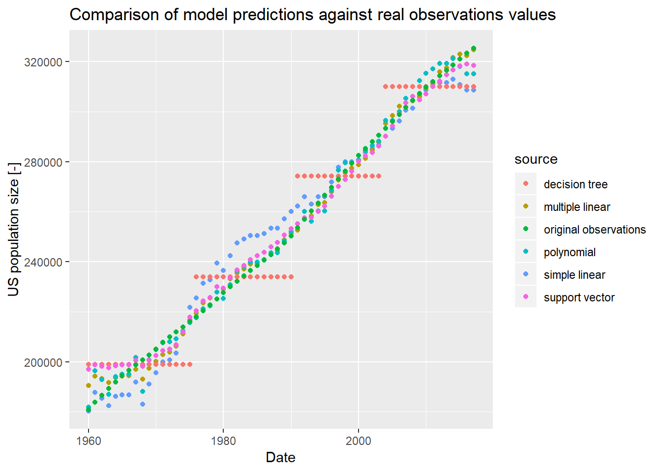
predictions_svr <- predict(predictor,data_df)모델 예측의 비교
저장된 예측 값이 있는 벡터를 사용하여 타임라인에서 다양한 예측 모델을 비교할 수 있습니다.
# construct ggplot friendly data frame
ggdata_df <- as.data.frame(matrix(nrow=nrow(data_df)*6,ncol=3))
colnames(ggdata_df) <- c("date","value","source")
ggdata_df$date <- rep(data_df$date,times=6)
ggdata_df$value <- c(predictions_slr,
                     predictions_mlr,
                     predictions_poly,
                     predictions_dtr,
                     predictions_svr,
                     data_df$population)
ggdata_df$source <- c(rep("simple linear", times=nrow(data_df)),
                      rep("multiple linear", times=nrow(data_df)),
                      rep("polynomial", times=nrow(data_df)),
                      rep("decision tree", times=nrow(data_df)),
                      rep("support vector", times=nrow(data_df)),
                      rep("original observations", times=nrow(data_df)))

# visualize
ggplot(ggdata_df) +
  geom_point(mapping = aes(x=date, y=value, color=source)) +
  ggtitle("Comparison of model predictions against real observations values") +
  xlab("Date") +
  ylab("US population size [-]")

최적화 및 시뮬레이션을 전문으로하는 산업 엔지니어 (R, Python, SQL, VBA)
Leave a Reply