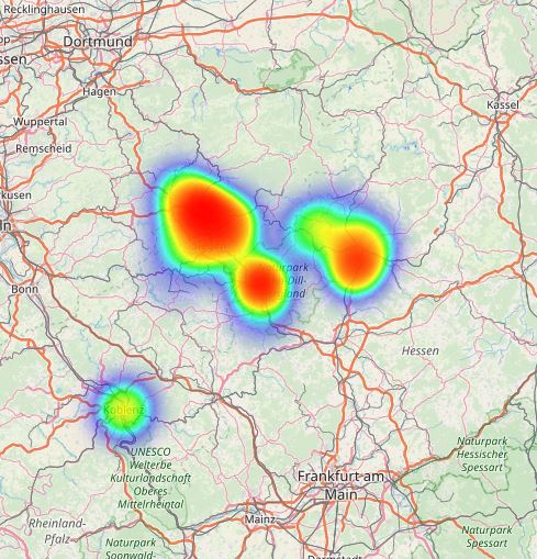
In a previous post I demonstrated how one can generate map-based heatmap distribution plots using the Leaflet package in R. In that example I implemented a function that sends locations as strings to a Open Street Map API and then receives latitude and longitude coordinates as return values in JSON-format.

In this post I will demonstrate how one can use the osmdata package to realize the geocoding part, without having to implement a “complicated” function.

First I define a set of cities and towns to use as locations; I add them to an empty data frame template with pre-defined header names as well as row and column counts

# defining a data frame tempalte to populate throughut geocoding process
data_df = as.data.frame(matrix(nrow=20,ncol=4))
colnames(data_df) = c("location","lat","long","values")

# adding city and town names as locations
data_df$location = c("Siegen, Germany",      #1
                     "Kreuztal, Germany",    #2
                     "Netphen, Germany",     #3
                     "Olpe, Germany",        #4 
                     "Freudenberg, Germany", #5
                     "Hilchenbach, Germany", #6
                     "Wilnsdorf, Germany",   #7
                     "Betzdorf, Germany",    #8
                     "Dillenburg, Germany",  #9
                     "Marburg, Germany",     #10
                     "Biedenkopf, Germany",  #11
                     "Koblenz, Germany",     #12
                     "Erndtebrück, Germany", #13
                     "Herborn, Germany",     #14
                     "Cölbe, Germany",       #15
                     "Haiger, Germany",      #16
                     "Krombach, Germany",    #17
                     "Wenden, Germany",      #18
                     "Betzdorf, Germany",    #19
                     "Münchhausen, Germany"  #20
                     )

Next, I geocode the locations using the osmdata package in R.

# importing osmdata package in R
library(osmdata)

# using getbb() function to geocode locations
for(i in 1:nrow(data_df)){
  coordinates = getbb(data_df$location[i])
  data_df$long[i] = (coordinates[1,1] + coordinates[1,2])/2
  data_df$lat[i] = (coordinates[2,1] + coordinates[2,2])/2
}

Now the data frame contains location names and geocoded longitude and latitude coordinates; in addition, I add some randomly distributed observation value per location (this will define the color intensity of the heatmap plot).

# adding randomly distributed values by location (uniform distribution)
data_df$values = runif(n = 20, min = 0, max = 100)

In a final step I generate a heatmap displaying the distribution of observation values by location, using Leaflet in R.

# importing leaflet, leaflet.extras and magrittr
library(leaflet)
library(leaflet.extras)
library(magrittr)

# creating a heat map for the burger search intensity according to Google trends
data_df %>%
  leaflet() %>% 
  addTiles() %>% 
  addProviderTiles(providers$OpenStreetMap.DE) %>% 
  setView(mean(data_df$long),mean(data_df$lat),8) %>%
  addHeatmap(lng=~long,lat=~lat,intensity=~values,max=100,radius=30,blur=20)

Linnart Felkl

Data scientist focusing on simulation, optimization and modeling in R, SQL, VBA and Python